Test of significance
The Statistical procedures, which are used to know whether differences under study are significant or non-significant are called test of significance. Some well known and commonly used test of significant are Z-test, t-test and F-test.
If \(\mu = H_0\) is the null hypothesis than
\(\mu \ne H_0\) or \(\mu > H_0\) or \(\mu < H_0\) is the alternative hypothesis.
Two-tailed and one-tailed hypothesis
Two sided alternative hypothesis has region of rejection in both tails of sampling distribution of test statistic and one sided alternative hypothesis has rejection region, either in the left tail or right tail of the sampling distribution of test statistic.
Errors in testing of hypothesis
As decision is based on sample information, so we are likely to make two types of errors in testing of hypothesis. These are
Type I Error is the error committed in rejecting a null hypothesis (\(\ H_0\)), when it is true.
Type II Error is the error committed in not rejecting a false null hypothesis.
Level of significance
It is the maximum probability of type I error; which is experimenter is willing to risk in testing a null hypothesis. It is denoted as $\alpha$.
For testing significance of difference between population mean and sample mean or between two sample means, either Z-test or t-test applied. A detailed and systematic explanation of Z-test and t-test can be found in the Blog Post Section
Analysis of variance and F-test
The method of partitioning total variation into components due to different causes is known as analysis of variance and the table showing the various mean squares together with the corresponding degree of freedom is called analysis of variance (ANOVA) table. The analysis of variance provides a ready means of testing significance of differences between class mean. Suppose we have two genotypes, A and B and data on a particular character were recorded for a number of plants in each genotypes. We want to know whether the genotypes differ with respect to that character or not. This can be done by both t-test and F-test. The F-test and t-test are in fact identical, since for a single degree of freedom of the numerator, the F ratio is identically equal to t2. However, F-test has a wider application than t-test as it also provides an overall test of several differences, whereas, t-test provides test of a single differences.
F-test
F-test is used to test whether the two independent estimates of population variance differ significantly or whether the two samples may be regarded as drawn from the normal population having the same variance. A detailed and systematic explanation of F-test can be found in the Blog Post Section
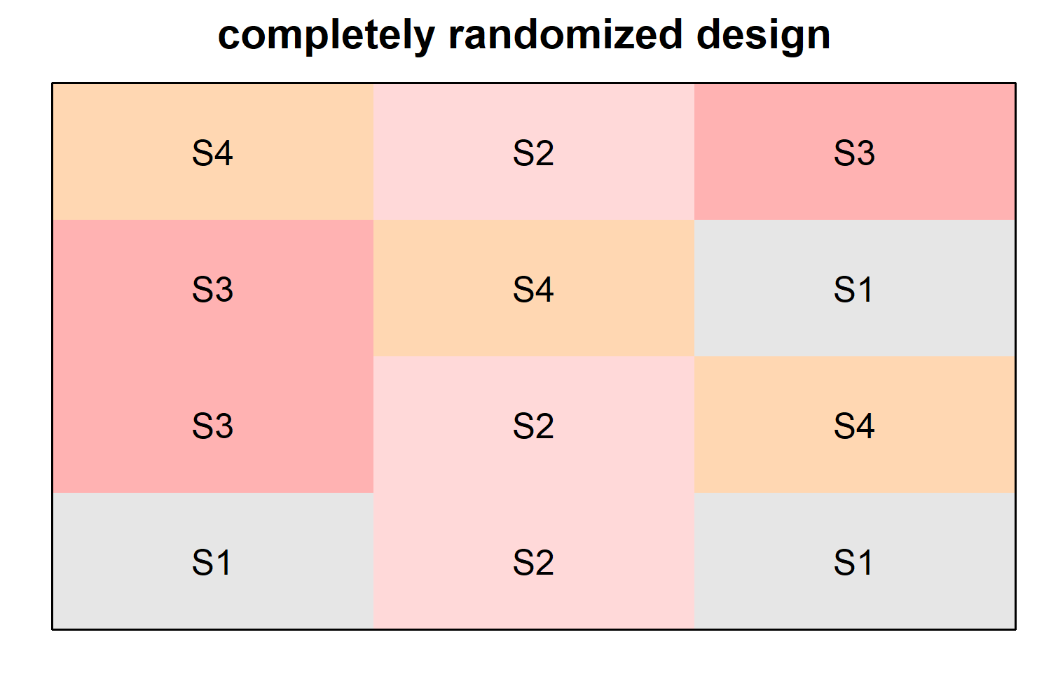
Completely Randomized Design (CRD)
The Completely Randomized Design (CRD) is the simplest experimental design. Treatments are assigned to experimental units purely at random, with no restrictions. It is the starting point for understanding all other designs (RCBD, Latin Square, Alpha-lattice) and remains widely used in controlled laboratory and greenhouse experiments. A comprehensive and structured explanation of CRD is available in the Blog Post Section
Comprehensive Analysis of Field Experiments in R
Field experiments constitute the foundation of applied agricultural research, providing a systematic approach for evaluating treatments under real-world conditions. These experiments are essential for generating reliable and scientifically valid conclusions regarding crop performance, input efficiency, and environmental interactions.
This guide presents a comprehensive analytical framework for conducting and interpreting field experiments using R. It begins with the fundamental Randomized Complete Block Design (RCBD), which is widely used for controlling field variability, and progressively advances to the more sophisticated Honeycomb Design, known for its efficiency in large-scale and heterogeneous environments.
Each section of this guide is carefully structured to include:
- a detailed explanation of the underlying statistical theory,
- the rationale behind the experimental layout and design structure,
- step-by-step implementation using R code, and
- thorough interpretation of the resulting outputs.
By integrating theoretical concepts with practical computational tools, this guide aims to equip researchers and students with a complete understanding of modern field experiment analysis.
Randomized Complete Block Design (RCBD)
Randomized Complete Block Design (RCBD) is one of the most widely used experimental designs in agricultural and biological research, particularly when there is known or suspected variability in the experimental field. In RCBD, the entire set of treatments is arranged into groups called blocks, where each block is relatively homogeneous with respect to environmental conditions such as soil fertility, moisture, or slope. Every treatment appears exactly once within each block, ensuring that comparisons among treatments are made under similar conditions. The allocation of treatments within each block is done randomly, which helps eliminate bias and ensures the validity of statistical inference.
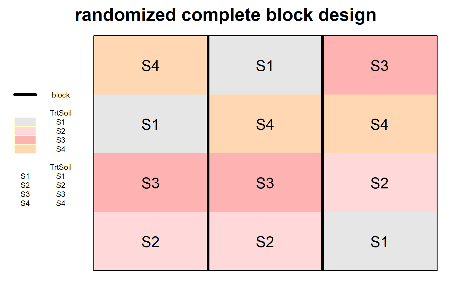
The primary advantage of RCBD lies in its ability to control variability by isolating the effect of nuisance factors through blocking. By accounting for block-to-block variation, the design reduces experimental error and increases the precision of treatment comparisons. The statistical analysis of RCBD is typically carried out using Analysis of Variance (ANOVA), where the total variation is partitioned into components due to treatments, blocks, and random error. If the treatment effect is found to be statistically significant, it indicates that the differences among treatment means are not due to chance alone. Overall, RCBD is highly efficient, simple to implement, and particularly suitable for field experiments where environmental heterogeneity exists in one direction. A detailed and systematic explanation of RCBD can be found in the Blog Post Section
Tip: If block F-value is not significant, blocking reduced power with no benefit — consider switching to CRD or using blocks as a random effect (mixed model).
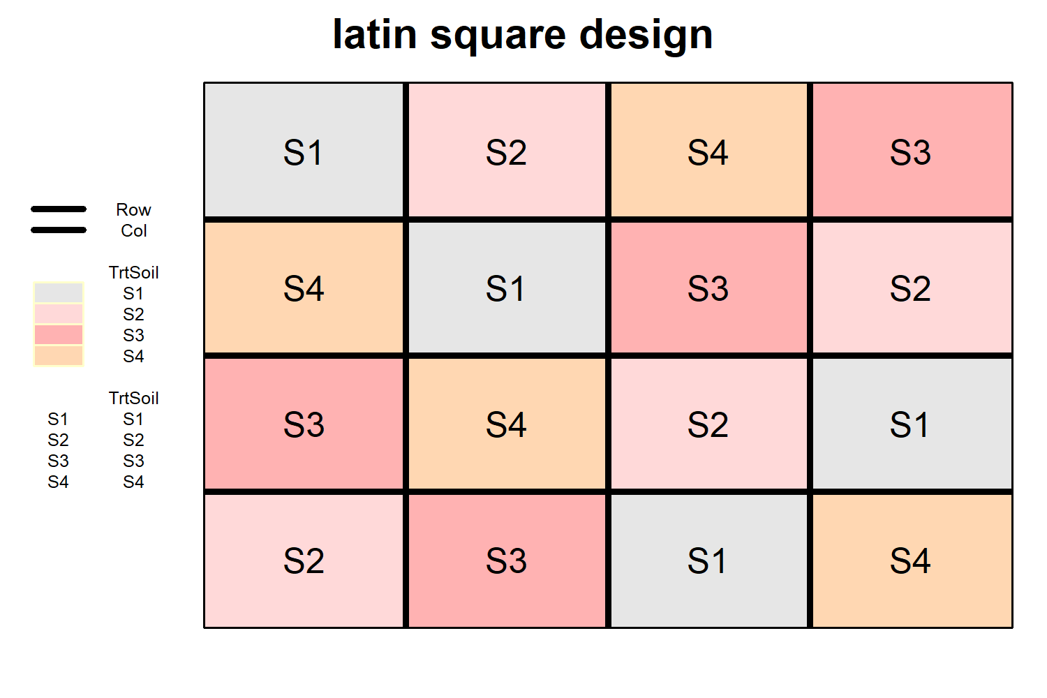
Latin Square Design (LSD)
Latin Square Design (LSD) is an experimental design used when there are two sources of variability that need to be controlled simultaneously, in addition to the treatment effects. It is particularly useful in agricultural and biological experiments where variation may occur in two directions—for example, soil fertility gradients running both north–south and east–west. The design arranges treatments in a square layout such that the number of treatments equals the number of rows and columns, and each treatment appears exactly once in every row and every column. This dual control of variation makes LSD more efficient than designs like RCBD when two directional sources of heterogeneity are present.
In a Latin Square Design with t treatments, the experimental field is divided into a t × t grid. Treatments are assigned in such a way that no treatment repeats within the same row or column, and randomization is applied to rows, columns, and treatment allocation to avoid bias. The statistical model includes effects for treatments, rows, and columns, allowing the total variation to be partitioned into these components along with random error. Analysis is typically performed using Analysis of Variance (ANOVA), where significance of treatment effects is tested after accounting for row and column variations. While LSD is highly efficient in controlling two sources of variability, it has limitations: it requires the number of treatments to equal the number of rows and columns, and missing data can complicate analysis. Despite these constraints, it remains a powerful design when experimental conditions vary in two directions. A detailed and systematic explanation Latin square Design can be found in the Blog Post Section
Constraint: Requires equal number of rows, columns, and treatments. Best for $p \leq 8$.
When treatments exceed manageable block size, incomplete block designs are preferred.
Alpha (α) Lattice Design
Alpha Lattice Design (α-lattice design) is an advanced incomplete block design widely used in agricultural research, particularly in plant breeding trials where a large number of treatments (e.g., genotypes) need to be evaluated efficiently. When the number of treatments becomes too large for designs like RCBD to remain effective, the experimental error increases due to within-block heterogeneity. The alpha lattice design addresses this issue by arranging treatments into incomplete blocks, each containing only a subset of the total treatments, while still maintaining an overall balanced structure across replications.
In this design, treatments are grouped into smaller blocks within each replication, and each replication contains all treatments, but distributed across multiple incomplete blocks. This structure helps control local variability more effectively than complete block designs, as comparisons are made within relatively homogeneous small blocks. The term “alpha” refers to the method of generating the design, which ensures near-balance in the occurrence and pairing of treatments across blocks. Although not all treatment pairs appear together in every block, the design is constructed so that statistical efficiency remains high.
 The analysis of an alpha lattice design is typically conducted using mixed-effects models, where blocks within replications are treated as random effects and treatments as fixed effects. In R, packages such as
 agricolae, lme4, or asreml are commonly used for analysis. The model accounts for variation due to replications, incomplete blocks, and residual error, allowing for more precise estimation of treatment effects. Overall, the alpha lattice design provides a powerful and flexible approach for handling large-scale experiments, improving accuracy while managing practical constraints such as land, labor, and environmental variability. A detailed and systematic explanation of Alpha (α) lattice Design can be found in the Blog Post Section
Augmented Design
Augmented Design (Augmented Block Design) is an experimental design widely used in agricultural research when a large number of new treatments (such as genotypes or varieties or clones) need to be evaluated but resources are insufficient to replicate all of them. In this design, a set of standard or check treatments is replicated across all blocks, while the new treatments are unreplicated and appear only once. The primary purpose of including replicated checks is to account for environmental variability across blocks and to provide a basis for adjusting the performance of unreplicated entries. This makes the design particularly useful in early-stage plant breeding trials, where hundreds of new lines must be screened efficiently.
 The structure of an augmented design typically involves dividing the experimental area into blocks, each containing all the check treatments and a subset of new treatments. Since the new entries are not replicated, their raw observations may be influenced by local environmental conditions. To address this, statistical adjustments are made using the performance of the replicated checks within each block, thereby improving the accuracy of comparisons. The analysis is commonly performed using analysis of variance (ANOVA) models tailored for augmented designs, or specialized methods available in statistical software like R (e.g., using packages such as agricolae). Overall, the augmented design provides a practical balance between resource constraints and the need for reliable evaluation, enabling researchers to efficiently identify promising treatments for further testing. A detailed and systematic explanation of Augmented Design can be found in the Blog Post Section
Partially Replicated (p-rep) Design
Partially Replicated Design (P-rep design) is a modern and highly efficient experimental design used in agricultural and plant breeding research when evaluating a large number of treatments under limited resources. In this design, only a subset of treatments is replicated, while the remaining treatments are included only once (unreplicated). This approach provides a practical balance between the need for replication (to estimate experimental error) and the constraint of limited field space, labor, or budget.
The key idea behind the P-rep design is to strategically select certain treatments—often referred to as checks or key entries—for replication across the experiment. These replicated treatments serve as a basis for estimating environmental variability and improving the precision of comparisons among all treatments. The unreplicated treatments, although observed only once, are statistically adjusted using information borrowed from the replicated entries through advanced modeling techniques. This makes the design particularly useful in early-stage breeding programs where hundreds or thousands of genotypes must be screened efficiently.
Unlike traditional designs such as RCBD or lattice designs, the P-rep design relies heavily on mixed-effects models for analysis. In these models, treatment effects may be considered fixed or random, and spatial or block effects are incorporated to account for field heterogeneity. In R, packages such as lme4, asreml, or SpATS are commonly used to analyze P-rep data, allowing for more accurate estimation of treatment performance through techniques like Best Linear Unbiased Prediction (BLUP).
Overall, the P-rep design offers significant advantages in terms of flexibility and resource efficiency. It enables researchers to evaluate a large number of treatments with improved precision compared to fully unreplicated designs, while avoiding the high cost of complete replication. However, careful planning and appropriate statistical analysis are essential to ensure reliable results. A detailed and systematic explanation of partial replicated design can be found in the Blog Post Section
Spatial Analysis with AR1 × AR1 Model
Spatial Analysis with AR1 × AR1 Model is a powerful statistical approach used in field experiments to account for spatial correlation among observations. In agricultural trials, experimental units (plots) are arranged in rows and columns, and measurements taken from nearby plots are often more similar than those farther apart due to underlying environmental gradients such as soil fertility, moisture, or management practices. Traditional designs like RCBD assume independence of errors, which is often violated in practice. The AR1 × AR1 (first-order autoregressive in both directions) model explicitly captures this spatial dependence, leading to more accurate estimation of treatment effects and improved statistical efficiency.
The AR1 × AR1 model assumes that correlation between observations decreases exponentially with distance in both the row direction (horizontal) and the column direction (vertical). It introduces two parameters: one for row-wise correlation (ρrow) and one for column-wise correlation (ρcol). The covariance structure of the residuals is modeled as the Kronecker product of two AR1 processes, one for rows and one for columns. This means that plots closer together have higher correlation, while those farther apart are less correlated. By incorporating this structure into the model, spatial trends that are not captured by blocking alone can be effectively controlled.
In practice, spatial analysis using the AR1 × AR1 model is implemented through mixed-effects models, where treatment effects are typically considered fixed, and spatially correlated residuals are modeled explicitly. In R, packages such as nlme, asreml, or SpATS are commonly used. For example, using nlme, one can specify a correlation structure with corAR1() for both rows and columns within a generalized least squares (GLS) or linear mixed model framework. The model estimates the spatial correlation parameters along with treatment effects, providing adjusted means that are less biased by field heterogeneity.
The advantages of using an AR1 × AR1 spatial model include reduced residual variance, increased precision of treatment comparisons, and better control of field trends compared to traditional designs. It is particularly beneficial in large field trials, plant breeding experiments, and situations where spatial variability is continuous rather than discrete. However, it requires careful model specification, sufficient data structure (regular grid layout), and appropriate software tools. Overall, spatial analysis using the AR1 × AR1 model represents a modern and robust approach to improving the quality and reliability of conclusions drawn from field experiments. A detailed and systematic explanation can be found in the Blog Post Section
Honeycomb Design
The Honeycomb (HC) design, developed by Fasoulas (1988) and later extended by Kyriakou and Fasoulas, is a field layout method used in plant breeding to improve the efficiency of mass selection under field variability. In this design, plants are arranged in a triangular (hexagonal) grid, so that each plant is surrounded by exactly six nearest neighbours at equal distances. This uniform spatial arrangement ensures that every plant experiences a similar level of competition, reducing environmental bias caused by uneven spacing or directional field effects.
The main idea of the HC design is to enhance the accuracy of selecting superior plants by controlling local competition and micro-environmental variation without requiring heavy replication. Because each plant is compared primarily with its immediate neighbours, breeders can better distinguish genetic performance from environmental noise. This makes the design particularly useful in early-generation selection, where large populations are evaluated and only a small number of superior individuals are retained for further breeding. A detailed and systematic explanation of honeycomb design can be found in the Blog Post
Factorial Experimental Design
A Factorial Experimental Design is an experimental strategy in which two or more factors are varied simultaneously, and all possible combinations of their levels are studied. This allows researchers to:
- Estimate the main effect of each factor
- Detect interactions between factors
- Draw conclusions over a wide range of conditions
- Use experimental resources more efficiently than one-factor-at-a-time (OFAT) experiments
Key principle: In a factorial design, every factor combination appears in the experiment — making it possible to separate the independent effect of each factor and assess how factors influence each other.
A detailed and systematic explanation of factorial experimental design can be found in the Blog Post
Split Plot Design
A Split Plot Design is a type of experimental design used when one or more factors are difficult or expensive to randomize at the level of individual experimental units. It is widely used in agricultural field trials, industrial experiments, and manufacturing studies.
The design partitions experimental units into two levels:
- Whole plots — the larger units to which the hard-to-change factor (the whole-plot factor) is applied
- Subplots — subdivisions of whole plots, to which the easy-to-change factor (the subplot factor) is applied
Key idea: Whole-plot factors are randomized among whole plots; subplot factors are randomized within each whole plot.
The blog provides a detailed and systematic explanation of split plot design, including its concepts, structure, and applications — Read the blog
Strip Plot Design
A Strip Plot Design (also called a Criss-Cross Design) is an experimental layout used when two factors are both difficult or costly to randomise at the level of individual plots. It is a natural extension of the split plot concept but treats both factors symmetrically — neither is nested within the other.
In a strip plot:
- Factor A (the row factor) is applied to horizontal strips running across each block
- Factor B (the column factor) is applied to vertical strips running down each block
- The intersection of a row strip and a column strip forms the experimental unit for the interaction A×B
Key idea: Both factors are randomised within blocks in perpendicular directions. The interaction is estimated at the smallest unit — the intersection cell — which typically has the highest precision.
The blog offers a comprehensive explanation of strip plot design, covering its structure, methodology, and practical applications — Read the blog.
Comparison of Designs
| Feature | RCBD | Alpha Lattice | p-rep | Honeycomb |
|---|---|---|---|---|
| Blocking direction | 1 | 2 (incomplete) | Spatial | Neighbour competition |
| # treatments | ≤ 30 | 20–1000 | 50–5000 | Unlimited |
| Replication | Complete | Partial | Partial (~30 %) | None (moving ring) |
| Error control | Moderate | Good | Excellent | Excellent |
| Primary use | Variety trials | Breeding stages | MET Stage 1 | Mass selection |
| Main R packages | agricolae |
agricolae, lme4
|
FielDHub, SpATS
|
FNN, custom |
Full Pipeline Utility Functions
# ── Wrapper: run any design ANOVA and return LSD groups ───────────────────
analyse_design <- function(data, yield_col = "Yield",
                           treat_col = "Treatment", ...) {
  extra_terms <- paste(..., collapse = " + ")
  formula_str <- paste(yield_col, "~", treat_col,
                       if (nchar(extra_terms)) paste("+", extra_terms) else "")
  model  <- aov(as.formula(formula_str), data = data)
  groups <- LSD.test(model, treat_col, console = FALSE)$groups
  list(anova = summary(model), groups = groups)
}

# Usage examples
analyse_design(rcbd_data,  "Block")               # RCBD
analyse_design(ls_long,    "Row", "Col")           # Latin Square
References & Further Reading
- Fasoulas, A. C. (1988). The Honeycomb Methodology of Plant Breeding. Thessaloniki.
- Kempton, R. A., & Fox, P. N. (Eds.) (1997). Statistical Methods for Plant Variety Evaluation. Chapman & Hall.
- Cullis, B. R., Smith, A. B., & Coombes, N. E. (2006). On the design of early generation variety trials with correlated data. JABES, 11(4), 381–393.
- Mramba, L. et al. (2019). FielDHub: A Shiny App for Design of Experiments in Life Sciences. CRAN.
- R Core Team (2026). R: A Language and Environment for Statistical Computing. R Foundation.